Linear Regression
We have already seen a little bit of how we do basic statistics using the summarize() function. Now we’ll expand on that by adding a few common statistical tests.
Linear Model
For many experiments, we are looking to understand if one variable is a good predictor for the other. We can get a visual of this by plotting both variables against one another, as we have done for our volumes. The straight line we draw through the points is our visual representation of a linear model. If one variable perfectly predicts the other, the line will have a slope of exactly 1. What we want to do is calculate the slope of our line to see how well our x-variable predicts our y-variable.
Mathematically, the calculation for our line is y = mx + b.
The code for that takes the general form: lm(y ~ x, data = your_data)
The y ~ x syntax will come up repeatedly when doing statistics in R. Here, y is always our dependent variable and x is our independent variable. The general way you can read that formula is “y varies by x” or “y as a factor of x”, meaning we want to see how y changes as we change x.
For our scatterplot, we plotted how bill length affects bill depth. Fill those in as our x and y variables in the function for creating a linear model.
This creates the model, then to see the information that we want from it, we will use the command summary() to show the model contents.
The resulting output is a little messy, but here’ the explanation:
“Call” shows us the formula for the model, “Residuals” shows the summary statistics for the residuals (the difference between observations and predictions), and “Coefficients” shows us our line information.
The “Coefficients” section is written as a table with variables as rows and values as the columns. The Estimate for (Intercept) shows the y-intercept, so “b” in y = mx + b. The Estimate for expected_vol shows the slope, so the “m” in y = mx + b.
We also see Error estimates for these values, a t-value, and a p-value which is written as Pr(>|t|). The t-value essentially gives you a measure of signal-to-noise, and the p-value tells you whether that result is significant. We often don’t care about the p-value for the Intercept, but it is informative for the expected_vol.
A Quick p-value Refresher
We use a p-value to help us determine if our result is so unlikely based on chance that we can reject our null hypothesis. A p-value tells us how unlikely our result is given the assumption that the null hypothesis is true. A very small p-value means it is very unlikely the null hypothesis is true, and therefore, we can conclude that there is some meaningful pattern or difference in our data.
In general in science, we use a cutoff value of 0.05 to say if a result is significant. If we get a value less than that our result is significant; if we get a value higher than that our result is not significantly different than what we would expect under random chance.
The asterisks are a code to quickly tell you whether a result is significant or not. More asterisks means a lower p-value, which means more significance. You may sometimes see that you have a repeated p-value of <2.2e-16. If you see this for multiple variables, it isn’t a mistake, that number is just the cutoff point at which R stops calculating things. Remembering scientific notation, you’ll note that that number is sixteen decimal places past zero, so it’s quite small.
The rest of the output describes the model overall. The “Residual standard error” tells you about how far off the model’s predictions are. The “Multiple” and “Adjusted R-squared” values tell you how much of your variation is explained by the predictive variable, the F-stastic tells you how much better your model is at predicting the outcome than if you had no model and just used the sample mean, and the p-value tells you if the F-statistic is signficant.
Multiple Linear Regression
We can add to our model to use several explanatory variables to predict our outcome. With this type of analysis you can use both quantitative and qualitative data, so we’ll add species to the model.
Any time you want to add additional predictors, you just add them to the end of the formula, so here’s the addition of species:
The part of the output that we care the most about is the highlighted portion. This gives us the coefficients for each explanatory variable and their signficance.
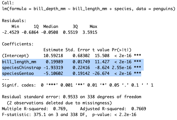 We see that all of our variables are highly signficant. Bill length has a slightly positive effect on bill depth (β = 0.19). For species, you may wonder why you only see Chinstrap and Gentoo, that’s because one group always is removed to be the comparator group. So these values are taking Adelie as the baseline and saying that if a penguin is a Chinstrap or Gentoo that will have a strong negative effect on bill depth as compared to Adelie.
Comparing Models
Both of these models we’ve built are ways to predict outcomes based on inputs. Since they have different inputs they will vary in how well they predict outcomes. There are many different tests to compare linear models and see which best fits the data, one of the most popular is the Akaike Information Criterion, or AIC, test. This gives an estimate of error for each of our models relative to the other.
The way you run an AIC in R is simply AIC(model1, model1). So our code would be:
The individual numbers in the output here don’t matter so much, what matters is how they relate to each other. You are looking for the model with the smaller AIC number because that shows it has a smaller amount of error in the model.
So, our model with both bill length and species is a better predictor for bill depth.
Practice
Does body weight predict flipper length? Is additionally factoring in species or sex important? Write code to find out.
Three predictor variables can be added to a model in the same way we did for two.