Exploring Your Data
Viewing Data
When you are using real RStudio and not this doc, you will see a variable object appear in the Environment after loading data.
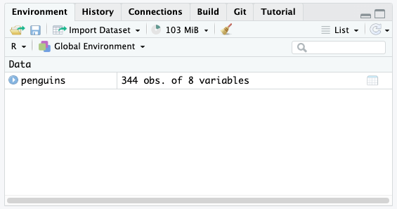
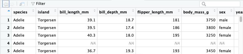
When you click that name (not the arrow, just the word), you can view the data and it will pop up in a spreadsheet format. Note, however, this spreadsheet is not directly editable.
glimpse()
A good way to get a quick look at your data is to use the glimpse() function. This will show you a list of the columns in your dataset, their data type, and the first few values in each column. This is often useful to make sure that your numerical data is actually read in as a number and not as a word or character. You can tell if something is numerical if it is the type dbl or int.
summary()
If you want a quick understanding of your data, the summary() function will tell you a lot about what each column contains. Run the following line of code and see what your output is:
You should see descriptive statistics for all of the numerical columns and some general info on the columns that aren’t numbers. For the numerical columns, you will see the mean, median, minimum value, maximum value, and the quartile range for your data. If any of your columns have missing values, you will also see how many NAs are present.
Working with Columns
To see the names of the columns in our dataset, we use the command colnames(). This will print out the name of each column.
$ Column Notation
There are a number of different ways to access individual columns, but we’ll start with $ notation. This is where you specify a column by typing the name of the dataset, $, and the column name. Here’s an example for the species column.
You should also notice that when you type the
$, R will pop up a helpful drop down list of all your column names. You can click those or press tab for the name to autocomplete.
That will print out all the values in the column (sometimes just some of the values, it has a cutoff point that it tells you). That might not be useful on its own, but it is useful when combined with functions.
Let’s use the function unique() to see all the possible values in the location column:
Making Variables from Columns
Columns can become their own objects in R by assigning them to a new variable name.
If we wanted to create a vector (basically a list) of all of the penguin weights, we could do that with this code:
Now we would see an object called weights appear in the Environment.
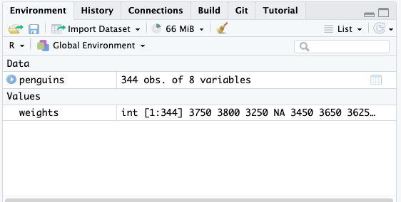
However, in this doc, when you run that code nothing will happen. You have saved it, but you haven’t displayed it, so no output will appear. The same is true for the console in RStudio. You will see the weights line appear in blue, but you won’t see the numbers print to the console. By running the name of an object we can see what its value is in the console:
Statistics on Single Columns
Similarly to how we did for the entire dataset, you can use the function summary() to find the descriptive stats just for a single column.
Or you can use mean() to find the average of a column. Try this:
You probably got an error for that one because if you have NAs in your data, the mean() function won’t be able to calculate the mean. We can fix that by adding an argument to the function.
If functions are like verbs, arguments can act as adverbs to slightly change the output of the function. For mean() we can add na.rm = TRUE to have R remove the missing values. Try that code again with the added argument.
? to Explain Functions
For any function, you can run ?function to see a help window that shows the documentation for that function. In RStudio, running ?mean will show you the following:
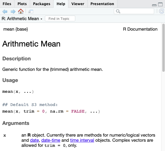
Here you can see the na.rm option as well as other components of how the function works.
Documentation for functions is sometimes very helpful and sometimes very confusing. It depends on who wrote it—sometimes people take the time to explain things well to a novice and sometimes they explain things only to experienced users. Usually, though, if you scroll to the bottom, there are example use cases that are the most helpful.