pop_data$country
pop_data$year
pop_data$lifeExpDatasets as Variable Objects
Once you’ve successfully run the read_csv() function you should see that the name pop_data appears in the Global Environment in the top right pane. When you click that name, you can view the data and it will pop up in a spreadsheet format. Note, however, this spreadsheet is not directly editable.
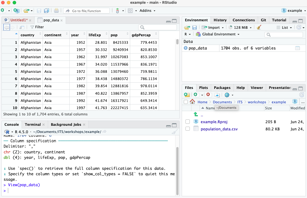
We have now read in the spreadsheet and saved the entire thing as an object called pop_data. An object is basically anything that holds data. That data can be a number, a word, a series of numbers, a paragraph, or an entire spreadsheet of data.
Assign <-
In order to create objects we use the <- symbol, which you can pronounce as “assign”. Anything you assign is an object. You will often hear the terms “object” and “variable” used interchangeably or smushed as “variable objects”. This is because when we’re analyzing data our objects typically are variables.
Columns are also variable objects
If your data is in what we call a “tidy format”, then all your columns will automatically be read in as their own variable objects inside the spreadsheet object. Tidy data refers to data where every column is a variable and every row is an observation.
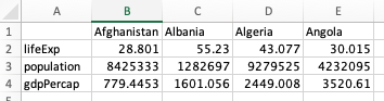
Here’s an example of untidy data, which we also sometimes call wide format data. It is often the easier way to initially write data down. A key signal to know if you have data in wide format is if there is an empty cell at the top left.
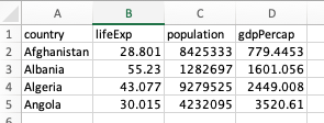
Here’s that same data as tidy data, also called long format data.
It’s fine to use wide format data when initially collecting data. We can easily convert it to tidy data where every column is a variable. (This will be an upcoming workshop.)
$ Notation for Columns
With this example we can now use country, year, and lifeExp as their own variables. There are a number of different ways to treat columns as variables, but we’ll start with $ notation. This is where you specify a column by typing the name of the dataset, $, and the column name. Here’s an example for the data above. Note that you have to type the column name exactly as it appears, including upper or lower case.
Running each of those lines will show me the contents of that column. Note again that R is case sensitive and I had to have the column names capitalized for that code to work.
If I wanted I could save each of those columns as their own variable object by assigning them to a name.
country_name <- pop_data$country
year <- pop_data$year
life_expectancy <- pop_data$lifeExp
Note that I can make up the name for whatever I want to assign them to. The only rules are that the names can’t have spaces (hence the underscore) and they can’t start with a number unless it is spelled out (5 vs five: only latter works).