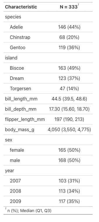
tbl_summary(na.omit(penguins))Summary Tables
A package that builds on {gt} that is also quite useful for tables is {gtsummary}. Unfortunately {gtsummary} also doesn’t play well with {webr}, but you can run this code in your version of R rather than the browser.
Basic Summary
We can easily create a summary table of all the penguin data by running the following line:
Note that I do need to remove NA values for this function to work properly.
Again, this looks pretty bad, but with the function tbl_summary we can make that look a lot nicer.
We can also specify specific columns that we’d like summary stats for. This code gives body mass statistics and it organizes them into columns based on what we specify, here they’re separated by species.
penguins |>
  select(species, sex, body_mass_g) |>
  tbl_summary(by = species)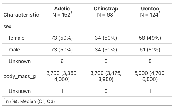
These are the automatic outputs, but there are many more arguments that can be added to augment things. We can filter out missing values by adding missing = "no" and change the statistic displayed to be mean and standard deviation rather than median and interquartile range.
penguins |>
  select(species, sex, body_mass_g) |>
  tbl_summary(by = species,
              missing = "no",
              statistic = all_continuous() ~ "{mean} ({sd})")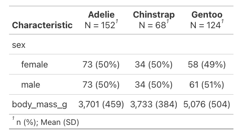
The syntax there is a little clunky, but it’s saying for any continuous values in the table calculate mean and sd and print them as “mean (sd)”.
Model Summaries
Where {gtsummary} really shines is taking the ugly output of model summaries and putting them in a readable format. Here’s a linear regression of body mass as a factor of bill length and depth. You’re maybe already familiar with the hard to interpret basic summary.
Pretty bad. A lot of text we don’t want and then other things like p-values that we’d like to be easily findable are a little buried.
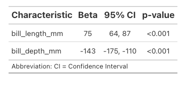
Here’s the same thing using the function tbl_regression:
tbl_regression(model)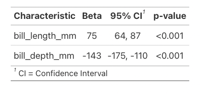
Much better! This stripped down version contains generally all the information people are wanting from these models, but you can change it to add in things like the intercept if you’d like less removed.
{gtsummary} has options for converting to the type of tables {gt} works with so you can access all the additional functions of {gt} like more formatting options. (The two packages are made by different people, so they don’t automatically use each other’s commands.)
Here we’re using as_gt from {gtsummary} with tab_options from {gt} to change the font sizes of the previous table.
tbl_regression(model) |>
  as_gt() |>
  tab_options(
    table.font.size = "small",
    column_labels.font.size = "16px"
  )