grad_raw <- read_csv("~/Documents/reed_data/grad_rates.csv")Loading & Viewing Data
We won’t go through loading data into R much in this tutorial because we’ll be using the interactive interface and data from a package. Loading data is sometimes one of the trickier steps for people if they aren’t familiar with file paths.
If you need help on loading files into R, go to the DataLab hours, or you can go to the loading data workshop that will walk you through how to add files on both the server and desktop versions of R.
Load Libraries Before Data
R comes with built in functions, but you can access many, many more by loading in libraries. Since R is open source, libraries can be written by anyone and can contain very specific functions. In order to load in the libraries you will use the function library() where the name of what you want goes inside the parentheses.
If you’re using a desktop version of R, you may need to install a library before you can use it. To do that you use the function install.packages(). You only install something once and then it’s on your computer until you intentionally remove it. But libraries need to be loaded every time you want use their functions. Think of installing packages like buying a book and loading libraries like getting the book off the shelf. You only need to buy it once (install.packages()), but every time you want to use it, you need to get it off the shelf (library()).
The words “package” and “library” refer to basically the same thing and are used interchangeably.
Workshop Library Setup
For this workshop, we will use the package {tidyverse}, which is like a super package with lots of other useful packages inside it, like {ggplot2} for graphing. We will also load a package from Github that contains Reed specific data. To load from Github, we’ll need to add one additional line. It’s not super important because you will mostly load data other ways, so it’s okay to not understand it.
# install from github
remotes::install_github("data-at-reed/reedr")

# load libraries
library(tidyverse)
library(reedr)
If you are just going to follow along in this web doc, you don’t need to run anything, it’s already set up to go. But if you’re running in your own version of R, copy over the code.
Add Data
Save Data as a Variable
In R, you can create variables and name them (mostly) whatever you would like. We’ll create a variable named raw_grad to store the graduation rates data from the {reedr} package.
If we were pulling this data from a file and not the package, that command would look more like this:
This uses a function to read in the data.
View Data
When you are using real RStudio and not this doc, you will see a variable object appear in the Environment after loading data.
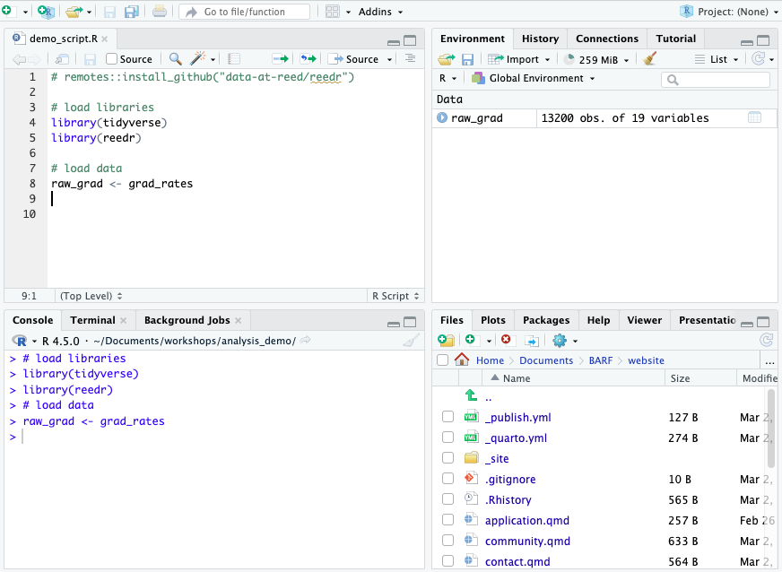
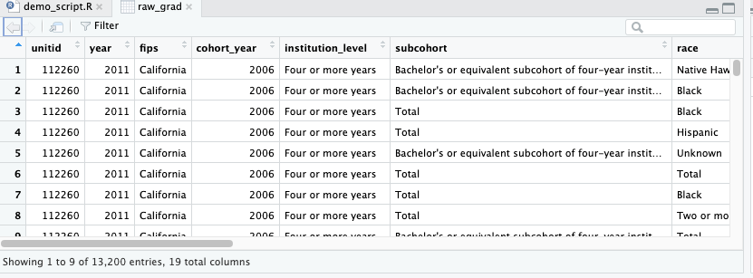
When you click that name (not the arrow, just the word), you can view the data and it will pop up in a spreadsheet format. Note, however, this spreadsheet is not directly editable.
glimpse()
A good way to get a quick look at your data is to use the glimpse() function. This will show you a list of the columns in your dataset, their data type, and the first few values in each column. This is often useful to make sure that your numerical data is actually read in as a number and not as a word or character. You can tell if something is numerical if it is the type dbl or int.
summary()
If you want a quick understanding of your data, the summary() function will tell you a lot about what each column contains. Run the following line of code and see what your output is:
You should see descriptive statistics for all of the numerical columns and some general info on the columns that aren’t numbers. For the numerical columns, you will see the mean, median, minimum value, maximum value, and the quartile range for your data. If any of your columns have missing values, you will also see how many NAs are present.